Faster partitioning for really big phylogenomic datasets
17 December 2015
Tweet
I’ve been working with the folks at 1Kite on estimating phylogenies from really really big phylogenomic datasets: think millions of sites for hundreds of taxa. One of the issues (there are many!) that we encounter with these datasets is that the usual methods are just not quick enough. And one of the usual methods is some software that I wrote called PartitionFinder.
PartitionFinder has been around for a while now, and we’ve been working on a complete overhaul for version 2. Apart from entirely rewriting the back-end of PartitionFinder I’ve been focussing on coming up with new algorithms that still find good partitioning schemes, but are fast enough to work well on datasets with millions of sites, thousands of taxa, and thousands of initial data blocks.
Most of the algorithms in PartitionFinder (except this one) work by starting with lots of user-defined data blocks, and then trying to figure out which ones evolved in sufficiently similar ways that they can be merged together. One method that we came up with to do this relatively quickly is something we called relaxed clustering. This method works by measuring a few things about the initial subsets in a partitioning scheme, and then focussing on pairs of subsets that look the most similar. From this set of similar subsets, we do a lot of calculations to figure out how each pairing changes the AICc/BIC score. The extra information we get from our measurements means that we don’t have to look at all possible combinations of data blocks, but instead we can focus on just those combinations that look promising.
The trouble is that this relaxed clustering algorithm (which I’ll call rcluster) still isn’t quick enough for the latest generation of enormous phylogenomic datasets. So I’ve been working on a faster version. The main problem with relaxed clustering is in the efficiency with which it uses processors. Let’s say I have an analysis where I tell the relaxed clustering algorithm to look at the 1000 most promising combinations of data blocks at each step, and I assign it 100 processors to do that. In the first step of the algorithm we look at 1000 combinations, and pick the best one (according to it’s AICc/BIC score), giving me a partitioning scheme with one fewer subsets than before. This will make good use of the 100 processors, particularly if we schedule jobs sensibly. The next step of the algorithm we’ll look at the 1000 best combinations again, but because not all of them are new combinations, we’ll have a lot less than 1000 jobs to do. We might have only 10 jobs. 10 jobs can never make good use of 100 processors. At best, we’ll be using 10% of them. To make things worse, some of the new models that are (rightly) popular in phylogenetics (like LG4X) can be tough to optimise, and because of that we often get one job that takes a lot longer than the others. This means that we can often be left waiting a long time for a single job to finish. So even though we have 100 processors available, we’re using just 1 for most of the time. In these cases, our efficiency can be shockingly low (<10%).
What we need is a new algorithm that’s more efficient. Turns out this is fairly simple. The sticking point on the old rcluster algorithm is that after the first step, we don’t get many jobs to do at each step, this means we have an upper limit on efficiency (the number of jobs / the number of available processors) which we don’t even hit when we have one job that takes much longer than all the rest. The solution is to find a way to do more jobs at once. To do this, I made a new algorithm that, instead of taking just the very best combination of subsets from the previous step, takes a whole lot of them. Let’s take the case above as an example. In the first step we’ll analyse 1000 combinations of subsets. In the old algorithm we’d take the combination that gives the biggest improvement to the AICc/BIC score. But in the new algorithm, I take the top 50% of all of the subset that improve the score. So, imagine that 600 of the 1000 combinations of subsets I looked at improve the AICc/BIC score. I’ll take the best 300 of those, giving me a partitioning scheme with 300 fewer subsets than before. In the next step of the algorithm, I again measure things about all the subsets and look at the best 1000 based on my measurements. Because so many of the starting subsets here are made up of new combinations of old subsets (300 of them, in fact) I’m likely to have a lot more jobs to do than in the old algorithm. I’ll call this algorithm rclusterf, with an ‘f’ for ‘fast’, but with the same name because much of the algorithm is similar. In fact, the old algorithm is just a special case of the new one.
To test the algorithm empirically, I used this data from the recent insect phylogenomics study. This dataset is big enough to be useful, but small enough to be manageable. It has 144 taxa, about half a million sites, and 2868 data blocks. I ran in partition finder with both algorithms, at a range of different settings. The only setting I changed was ‘rcluster-max’, which specifies how many combinations of subsets we should examine at each step of the algorithm. Here are the results:
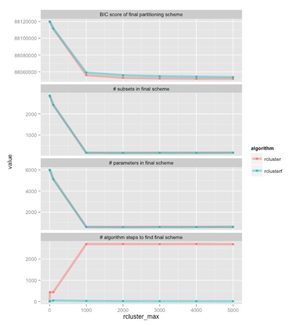
Let’s start at the bottom. This shows how many algorithm steps it takes for each algorithm (old one in pink, new one in blue) to find the best partitioning scheme they can. Once rcluster-max is 1000, the old algorithm consistently takes about 2700 steps, while the new one takes about 12. In the old algorithm, that’s 2700 times that we have to hang around waiting for one or a small number of jobs to finish. The upshot is that the new algorithm is going to be a lot faster, even though each step of the new rclusterf algorithm will take longer than the old rcluster algorithm (because we’re looking at new combinations of subsets at each step).
The top three graphs show something very encouraging: the two algorithms tend to find very similar partitioning schemes. They have about the same number of subsets in them, and about the same number parameters. There are minor differences, but given what we know about the effects of these kinds of differences on phylogenetic inference, I’d be very surprised if these differences made any appreciable difference to the trees that we would infer from this data. The top shows that the two algorithms (old one in pink, new one in blue) find partitioning schemes with very similar BIC scores (remember, lower BIC scores are better). The rclusterf algorithm is consistently a worse for a given setting of rcluster_max, but given that it’s a lot quicker we can probably (I haven’t checked) estimate a partitioning with a better BIC score in a given amount of time if we use the rclusterf algorithm rather than the rcluster algorithm, just by setting rcluster-max a bit higher.
What I need to do now is compare the trees you get from the partitioning schemes (which for me is the real acid test), and measure exactly how long each analysis takes when you do it from scratch (the analyses I show here rely on a lot of stored results, so I can’t get absolute timings). But for now, the new algorithm looks encouraging as a way of selecting partitioning schemes when you have really huge datasets and want results in a reasonable amount of time. If you want to try it out, you can find it here.
I’ve been working with the folks at 1Kite on estimating phylogenies from really really big phylogenomic datasets: think millions of sites for hundreds of taxa. One of the issues (there are many!) that we encounter with these datasets is that the usual methods are just not quick enough. And one of the usual methods is some software that I wrote called PartitionFinder.
PartitionFinder has been around for a while now, and we’ve been working on a complete overhaul for version 2. Apart from entirely rewriting the back-end of PartitionFinder I’ve been focussing on coming up with new algorithms that still find good partitioning schemes, but are fast enough to work well on datasets with millions of sites, thousands of taxa, and thousands of initial data blocks.
Most of the algorithms in PartitionFinder (except this one) work by starting with lots of user-defined data blocks, and then trying to figure out which ones evolved in sufficiently similar ways that they can be merged together. One method that we came up with to do this relatively quickly is something we called relaxed clustering. This method works by measuring a few things about the initial subsets in a partitioning scheme, and then focussing on pairs of subsets that look the most similar. From this set of similar subsets, we do a lot of calculations to figure out how each pairing changes the AICc/BIC score. The extra information we get from our measurements means that we don’t have to look at all possible combinations of data blocks, but instead we can focus on just those combinations that look promising.
The trouble is that this relaxed clustering algorithm (which I’ll call rcluster) still isn’t quick enough for the latest generation of enormous phylogenomic datasets. So I’ve been working on a faster version. The main problem with relaxed clustering is in the efficiency with which it uses processors. Let’s say I have an analysis where I tell the relaxed clustering algorithm to look at the 1000 most promising combinations of data blocks at each step, and I assign it 100 processors to do that. In the first step of the algorithm we look at 1000 combinations, and pick the best one (according to it’s AICc/BIC score), giving me a partitioning scheme with one fewer subsets than before. This will make good use of the 100 processors, particularly if we schedule jobs sensibly. The next step of the algorithm we’ll look at the 1000 best combinations again, but because not all of them are new combinations, we’ll have a lot less than 1000 jobs to do. We might have only 10 jobs. 10 jobs can never make good use of 100 processors. At best, we’ll be using 10% of them. To make things worse, some of the new models that are (rightly) popular in phylogenetics (like LG4X) can be tough to optimise, and because of that we often get one job that takes a lot longer than the others. This means that we can often be left waiting a long time for a single job to finish. So even though we have 100 processors available, we’re using just 1 for most of the time. In these cases, our efficiency can be shockingly low (<10%).
What we need is a new algorithm that’s more efficient. Turns out this is fairly simple. The sticking point on the old rcluster algorithm is that after the first step, we don’t get many jobs to do at each step, this means we have an upper limit on efficiency (the number of jobs / the number of available processors) which we don’t even hit when we have one job that takes much longer than all the rest. The solution is to find a way to do more jobs at once. To do this, I made a new algorithm that, instead of taking just the very best combination of subsets from the previous step, takes a whole lot of them. Let’s take the case above as an example. In the first step we’ll analyse 1000 combinations of subsets. In the old algorithm we’d take the combination that gives the biggest improvement to the AICc/BIC score. But in the new algorithm, I take the top 50% of all of the subset that improve the score. So, imagine that 600 of the 1000 combinations of subsets I looked at improve the AICc/BIC score. I’ll take the best 300 of those, giving me a partitioning scheme with 300 fewer subsets than before. In the next step of the algorithm, I again measure things about all the subsets and look at the best 1000 based on my measurements. Because so many of the starting subsets here are made up of new combinations of old subsets (300 of them, in fact) I’m likely to have a lot more jobs to do than in the old algorithm. I’ll call this algorithm rclusterf, with an ‘f’ for ‘fast’, but with the same name because much of the algorithm is similar. In fact, the old algorithm is just a special case of the new one.
To test the algorithm empirically, I used this data from the recent insect phylogenomics study. This dataset is big enough to be useful, but small enough to be manageable. It has 144 taxa, about half a million sites, and 2868 data blocks. I ran in partition finder with both algorithms, at a range of different settings. The only setting I changed was ‘rcluster-max’, which specifies how many combinations of subsets we should examine at each step of the algorithm. Here are the results:
Let’s start at the bottom. This shows how many algorithm steps it takes for each algorithm (old one in pink, new one in blue) to find the best partitioning scheme they can. Once rcluster-max is 1000, the old algorithm consistently takes about 2700 steps, while the new one takes about 12. In the old algorithm, that’s 2700 times that we have to hang around waiting for one or a small number of jobs to finish. The upshot is that the new algorithm is going to be a lot faster, even though each step of the new rclusterf algorithm will take longer than the old rcluster algorithm (because we’re looking at new combinations of subsets at each step).
The top three graphs show something very encouraging: the two algorithms tend to find very similar partitioning schemes. They have about the same number of subsets in them, and about the same number parameters. There are minor differences, but given what we know about the effects of these kinds of differences on phylogenetic inference, I’d be very surprised if these differences made any appreciable difference to the trees that we would infer from this data. The top shows that the two algorithms (old one in pink, new one in blue) find partitioning schemes with very similar BIC scores (remember, lower BIC scores are better). The rclusterf algorithm is consistently a worse for a given setting of rcluster_max, but given that it’s a lot quicker we can probably (I haven’t checked) estimate a partitioning with a better BIC score in a given amount of time if we use the rclusterf algorithm rather than the rcluster algorithm, just by setting rcluster-max a bit higher.
What I need to do now is compare the trees you get from the partitioning schemes (which for me is the real acid test), and measure exactly how long each analysis takes when you do it from scratch (the analyses I show here rely on a lot of stored results, so I can’t get absolute timings). But for now, the new algorithm looks encouraging as a way of selecting partitioning schemes when you have really huge datasets and want results in a reasonable amount of time. If you want to try it out, you can find it here.