Calculating and interpreting gene- and site-concordance factors in phylogenomics
14 December 2018
Tweet
We (Minh Bui, Matt Hahn, and I) have just published a new version of IQ-TREE that calculates gene- and site-concordance factors for phylogenetic analyses. The application note describes the calculations, but doesn’t have much space for guidance on how to use and interpret the concordance factors. So that’s what this post is for. A gist with all the R code used for this post, as well as all the input and output files you need, is here.
The dataset contains 54 genes split into 88 individual loci (individual introns and exons). Since we shouldn’t expect different regions of a single gene to share a gene tree (e.g. see this paper, I’ll treat each of the 88 loci separately. If you want to follow along, the nexus file with loci specified as character sets is available here.
The first step is just to look at the concordance factors on the tree. To do this, just load the output tree (concord.cf.tree) in any tree viewer. In this tree, each branch label shows bootstrap / gCF / sCF. Here’s one part of the bird tree, showing penguins and tubenoses:
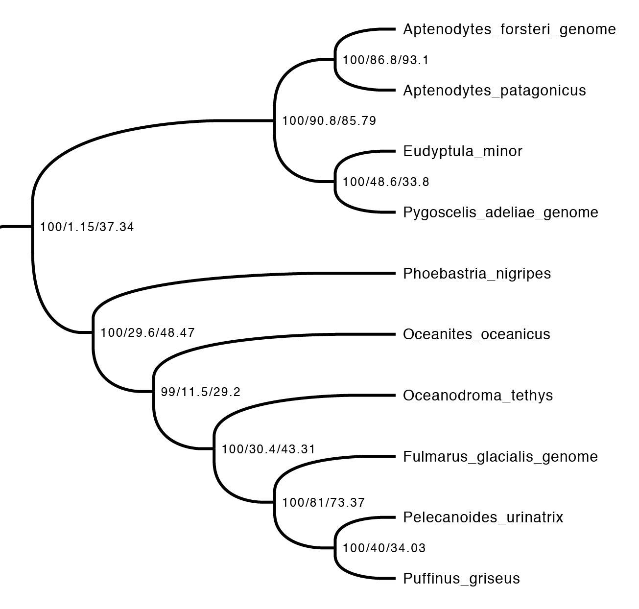
This part of the tree immediately illustrates the most important point: bootstraps and concordance factors are giving you very different information about each branch in the tree. Just take a look at how different the three numbers can be! For example, the deepest split has 100% bootstrap support, but a gCF of 1.15% and an sCF of 37.34%. This means that just a single one of the 88 single locus trees contains this grouping, while just over a third of the sites informative for this branch support it. Why are the numbers so different? The high bootstrap value tells us that the sampling variance for this branch is low. This is exactly what we expect with big datasets (this one is ~130K sites, which isn’t particularly big by today’s standards) – I’ll show exactly why in the next section. The gCF is probably low for two reasons: our ability to resolve single locus trees is limited because they’re short (and this is a short branch in the tree, which makes things worse), and many of the loci contain genuinely conflicting signal. The sCF helps us dig deeper here – the sCF for this node is ~37%, suggesting that the low gCF is a combination of both factors. Roughly speaking we expect the gCF and sCF to be similar if the only thing causing a low gCF is genuine discordant signal in the single locus trees. If the gCF values are affected by other processes (e.g. stochastic error from limited information), then gCF values can be a lot lower than sCF values. An sCF of 37% shows that there is not overwhelming support for any particular resolution of this branch. A sensible biological interpretation here would be that this resolution of the tree is a good best guess for the species tree, but that there is plenty of conflicting signal meaning that: (i) I wouldn’t bet my house on this resolution of the species tree; (ii) even if this is the correct resolution, there’s probably a lot of conflicting signal in the gene trees from processes like incomplete lineage sorting.
Here’s the code, and below is the plot (I load lots of libraries because I do other things with the data later on):
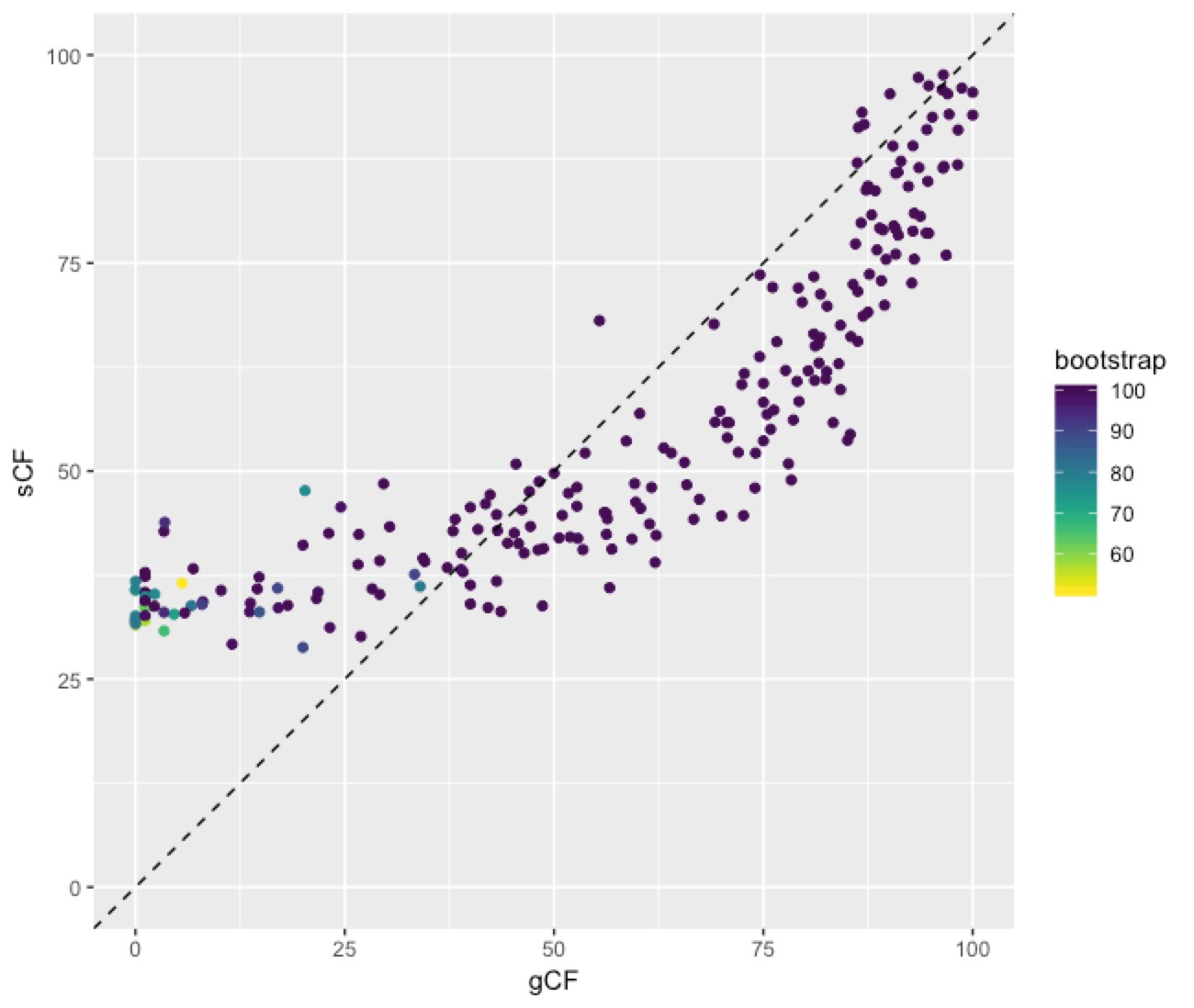
This plot shows a few important things. First, low bootstrap values (bright colours) coincide with the lowest gCF and sCF values, as expected. You can only get a low bootstrap value when the there’s very limited information on that branch in the alignment. And if there’s very little information, there will be very few sites (and therefore genes) that can support a branch. Second, bootstrap values max out at 100% pretty quickly, even for very low gCF and sCF values. Third, sCF values have a minimum of ~30%, but gCF values can go all the way to 0%. This is because sCF values are calculated by comparing the three possible resolutions of quartet around a node, so when the data are completely equivocal about these resolutions, we expect an sCF value of 33%. gCF values, on the other hand, are calculated from full gene trees, such that there are many more than 3 possible resolutions around a node, and the gCF value can be as low as 0% if no single gene tree contains a branch that’s present in the reference tree. This can happen (and does, in this bird dataset) when a combination of biology and stochastic error leads to a lot of gene-tree discordance.
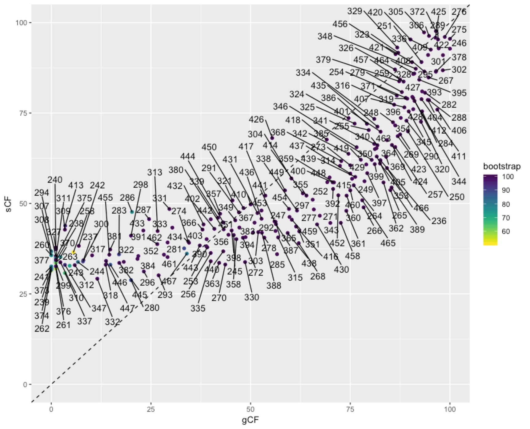
In some cases you might want to identify individual nodes in the plot above. This is easy enough to do with ggrepel():
To get at the discordance factors for the deepest split in the tree above, we need to figure out the ID of the branch. You can do this by loading the concord.cf.branch file into your tree viewer. In this tree the branch labels are ID numbers that are used in various other output files that IQ-TREE produces. In this case, the branch we are interested in has ID 327. Now we can look up some more details on that branch in the file concord.cf.stat. You can do this straight from the text file, using excel, or in R. I’ll do it in R:
which gives us:
We can see a number of things from this. First, the branch is very short, and that’s probably most of the reason for the low gCF (short branches are hard to resolve, particularly with short loci). This is confirmed by the fact that although 87 of the 88 single locus trees could have contained this branch (gN = 87 in the table, meaning that 87 of the 88 gene trees could have contained that branch; these gene trees are called decisive in the preprint), only 1 of them did (1.15% of 87 is 1). Three other single locus trees supported a second resolution of the four clades around that branch (gDF1 = 3.45%, corresponding to 3 trees), and none supported the third resolution (gDF2 = 0%). The remaining 83 out of the 87 gene trees had a topology that wasn’t any one of the three possible arrangements of the four clades around this branch, which is a typical signal of noisy single locus trees. This highlights another important point – the most common resolution of this branch in the gene trees is NOT the one we see in the ML concatenated tree. There are at least two reasons this might be the case – we might be in the anomaly zone, or it might be that the informative sites for this tree are scattered around in all the noisy genes, such that individual gene trees really aren’t giving us much useful information here. The sCF and sDF values suggest that the latter explanation is true (see below). In itself, this highlights a limitation of methods that look to build a species tree from pre-estimated gene trees: when the gene trees are noisy, these methods will struggle.
The sCF is particularly useful when the single locus trees are noisy. When interpreting sCF values, it’s important to note that unlike gCF values the three sCF values sum to 100%, because we ask for each site which of the three possible quartets around a given branch it supports. For our branch of interest (branch 327), the sCF (corresponding to the arrangement in the tree above) is 37%, the sDF1 (one of the other arrangements) is 30%, and the sDF2 (the final arrangement) is 33%. The sN tells us that there were ~350 decisive sites for this branch (the number isn’t an integer because it’s calculated as an average across many possible quartets, more information on this is in the preprint). That means that about 131 sites support the resolution in the tree above (sCF), while 114 support the next best resolution (sDF2). Intuitively, 131 sites vs. 114 sites seems like a small difference, and that’s why we think that knowing the sCF value (~37% in this case) tells you something useful that a bootstrap does not (the bootstrap is 100% in this case).
But how can the bootstrap be so high, when the sCF is so low? This is because bootstrap values are measuring sampling variance, while the sCF is measuring the observed variance in the original data. This difference is important, and highlights why in many cases (especially for large phylogenomic datasets) gCF and sCF values are a useful complement to bootstrap values. Specifically, it makes it explicit that a very low sampling variance (e.g. 100% bootstrap support) tells you very little about the underlying variation in your data. An analogy might be useful here: imagine you collect height data from 1 million individuals in a population. Let’s say your data show that individuals can range from 4 feet tall to 10 feet tall, and that the distribution is almost uniform. If you calculate the mean of this distribution, and then recalculate it again and again from bootstrapped samples of your dataset, you’ll see that your sampling variance on the mean is very low because you have such a big dataset. But if you were to measure the variance of your raw data, you’d see that this is very high. A low sampling variance on the mean is analogous to a high bootstrap value (which indicates a low sampling variance on a branch in tree), and a high observed variance is like a low sCF value (which indicates high variance in the support that sites give for the correct resolution of this branch).
Felsenstein’s 1985 bootstrap paper gives us a formula which tells us that we should expect very high bootstrap support if we have 131 vs. 114 sites competing to resolve a single branch. Indeed, it says that the bootstrap support for a difference of 17 sites in an alignment of length 137324 should be 99.999% in favour of the resolution with the most supporting sites. Regardless, these sCF values tell us that despite a bootstrap support of 100%, the underlying data contain a lot of discordance (almost the maximum possible amount) around this one branch.
This produce a tibble in which the last two columns are the p values we’re interested in. We can look at just those that interest us like this:
which shows that a lot of branches reject the ILS assumptions, assuming our chi-squared approach is accurate (which it won’t be among sites in a single gene because of linkage disequilibrium, so be careful with these p values):
The table also happens to contain some intriguing disagreements between gCF and sCF values. For example, row 45 (branch ID 280) has a gCF of 20% (which is very low), a gDF1 of 0% and a gDF2 of ~15%. The latter two numbers are far from even, and the p value of the chi-square test (gEF_p) is <<0.05. But the sites tell a different story: the sCF is 29% (again, very low), the sDF1 is 36%, and the sDF2 is 35%. What’s odd here is that the resolution in the ML tree is supported by many fewer sites than either of the two competing resolutions. My guess is that the site likelihoods are such that the resolution in the ML tree wins out. But tellingly, the bootstrap support here is low-ish (89%), as we might expect when the sCF is lower than one or both of the sDF values.
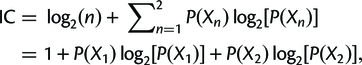
where P(X1) = X1/(X1 + X2), P(X2) = X2/(X1 + X2), and P(X1) + P(X2) = 1.
X1 is just the number of gene trees supporting the resolution in the reference tree, and X2 is the number of gene trees supporting the next best resolution.
For gCF we can’t do this exactly, but if we’re willing to assume that the next-most-common resolution of a branch is one of either gDF1 or gDF2, we can calculate the gene IC, which I’ll call gIC. We can use the site concordance and discordance values to do something similar for sites. In this case, we use the same formula, but simply use site counts instead of gene counts. I’ll call this sIC. Note that because we do sites on quartets, and there are only three possible resolutions, we can guarantee that the sIC we calculate will have the most common alternative resolution as X2. Here’s how to calculate gIC and sIC:
The IC is an interesting measure, but it throws out a lot of information (ALL of the other possible resolutions). For the sites, I think we can do better than calculating the sIC as above. The IC is inspired by measures of entropy, and in the case of sites, we can just calculate the entropy directly from the three values in sCF, sDF1, and sDF2. If these all have equal values (i.e. they all represent ~33% of the sites), this will give the maximum possible entropy of 1.098612. So, we could report this directly (let’s call this sENT), or we could convert it into a measure of certainty that scales between 0 (when there is maximum entropy) and 1 (when there is minimum entropy). I’ll call this sENTC for entropy certainty. That’s a horrible name. I’m not suggesting anyone use this measure, I’m only calculating it for comparison, and I’d love to think of a good name but I’m about to go on holiday.
Now we have more measures than anybody wants. But we can at least see the extent to which they measure different things by plotting them all against each other:
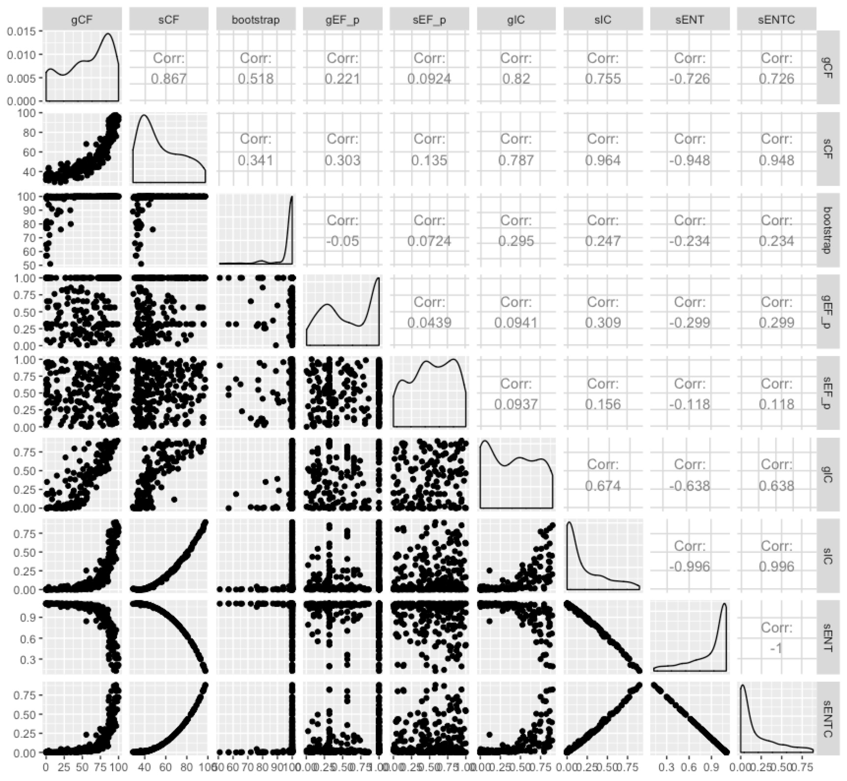
Some of them are highly correlated, and it seems fairly clear that the entropy-based measures don’t tell us a whole lot more than the concordance factors in most cases. I like the concordance factors because they have such an intuitive interpretation - the proportion of genes (gCF) or sites (sCF) that are concordant with any particular branch in your tree.
We (Minh Bui, Matt Hahn, and I) have just published a new version of IQ-TREE that calculates gene- and site-concordance factors for phylogenetic analyses. The application note describes the calculations, but doesn’t have much space for guidance on how to use and interpret the concordance factors. So that’s what this post is for. A gist with all the R code used for this post, as well as all the input and output files you need, is here.
The data
For this post, I’ll focus on an alignment of 88 loci (137324 sites) and 235 bird species from a recent paper. The bird tree is interesting because there are lots of studies that produce trees with ~100% bootstrap support on almost every node, but the topologies often disagree. In cases like these, understanding the variation in the underlying data can be very useful. And that’s exactly what gene- and site-concordance factors (which I’ll call gCF and sCF from here) are for.The dataset contains 54 genes split into 88 individual loci (individual introns and exons). Since we shouldn’t expect different regions of a single gene to share a gene tree (e.g. see this paper, I’ll treat each of the 88 loci separately. If you want to follow along, the nexus file with loci specified as character sets is available here.
How to calculate concordance factors in IQ-TREE
We start by estimating the gCF and sCF values for each branch on a tree produced by maximum likelihood on a concatenated alignment. This takes just three steps in IQ-TREE: estimate a concatenated tree; estimate the single-locus trees; and then calculate the gCF and sCF values using the concatenated tree as a reference tree (there’s a full tutorial here). This is a big dataset, so the analysis takes a while. You can view and download the relevant output files here if you’re interested.Using concordance factors to understand your data
The first step is just to look at the concordance factors on the tree. To do this, just load the output tree (concord.cf.tree) in any tree viewer. In this tree, each branch label shows bootstrap / gCF / sCF. Here’s one part of the bird tree, showing penguins and tubenoses:
This part of the tree immediately illustrates the most important point: bootstraps and concordance factors are giving you very different information about each branch in the tree. Just take a look at how different the three numbers can be! For example, the deepest split has 100% bootstrap support, but a gCF of 1.15% and an sCF of 37.34%. This means that just a single one of the 88 single locus trees contains this grouping, while just over a third of the sites informative for this branch support it. Why are the numbers so different? The high bootstrap value tells us that the sampling variance for this branch is low. This is exactly what we expect with big datasets (this one is ~130K sites, which isn’t particularly big by today’s standards) – I’ll show exactly why in the next section. The gCF is probably low for two reasons: our ability to resolve single locus trees is limited because they’re short (and this is a short branch in the tree, which makes things worse), and many of the loci contain genuinely conflicting signal. The sCF helps us dig deeper here – the sCF for this node is ~37%, suggesting that the low gCF is a combination of both factors. Roughly speaking we expect the gCF and sCF to be similar if the only thing causing a low gCF is genuine discordant signal in the single locus trees. If the gCF values are affected by other processes (e.g. stochastic error from limited information), then gCF values can be a lot lower than sCF values. An sCF of 37% shows that there is not overwhelming support for any particular resolution of this branch. A sensible biological interpretation here would be that this resolution of the tree is a good best guess for the species tree, but that there is plenty of conflicting signal meaning that: (i) I wouldn’t bet my house on this resolution of the species tree; (ii) even if this is the correct resolution, there’s probably a lot of conflicting signal in the gene trees from processes like incomplete lineage sorting.
How concordance factors relate to each other and to bootstraps
More generally, we can look at the links between bootstrap, gCF, and sCF across all nodes of the tree. This is simple to do in R, because IQ-TREE outputs a tab-delimited file that’s easy to read called concord.cf.stat. This file has one row per branch in the tree, and gives a lot of details on the statistics for each branch.Here’s the code, and below is the plot (I load lots of libraries because I do other things with the data later on):
This plot shows a few important things. First, low bootstrap values (bright colours) coincide with the lowest gCF and sCF values, as expected. You can only get a low bootstrap value when the there’s very limited information on that branch in the alignment. And if there’s very little information, there will be very few sites (and therefore genes) that can support a branch. Second, bootstrap values max out at 100% pretty quickly, even for very low gCF and sCF values. Third, sCF values have a minimum of ~30%, but gCF values can go all the way to 0%. This is because sCF values are calculated by comparing the three possible resolutions of quartet around a node, so when the data are completely equivocal about these resolutions, we expect an sCF value of 33%. gCF values, on the other hand, are calculated from full gene trees, such that there are many more than 3 possible resolutions around a node, and the gCF value can be as low as 0% if no single gene tree contains a branch that’s present in the reference tree. This can happen (and does, in this bird dataset) when a combination of biology and stochastic error leads to a lot of gene-tree discordance.
In some cases you might want to identify individual nodes in the plot above. This is easy enough to do with ggrepel():
Digging deeper using discordance factors
We can dig deeper into the node that splits penguins and tubenoses using other output from IQ-TREE that tells us about discordance factors. A discordance factor relates to the proportion of genes (gDF) or sites (sDF) that support a different resolution of the branch we’re interested in.To get at the discordance factors for the deepest split in the tree above, we need to figure out the ID of the branch. You can do this by loading the concord.cf.branch file into your tree viewer. In this tree the branch labels are ID numbers that are used in various other output files that IQ-TREE produces. In this case, the branch we are interested in has ID 327. Now we can look up some more details on that branch in the file concord.cf.stat. You can do this straight from the text file, using excel, or in R. I’ll do it in R:
which gives us:
We can see a number of things from this. First, the branch is very short, and that’s probably most of the reason for the low gCF (short branches are hard to resolve, particularly with short loci). This is confirmed by the fact that although 87 of the 88 single locus trees could have contained this branch (gN = 87 in the table, meaning that 87 of the 88 gene trees could have contained that branch; these gene trees are called decisive in the preprint), only 1 of them did (1.15% of 87 is 1). Three other single locus trees supported a second resolution of the four clades around that branch (gDF1 = 3.45%, corresponding to 3 trees), and none supported the third resolution (gDF2 = 0%). The remaining 83 out of the 87 gene trees had a topology that wasn’t any one of the three possible arrangements of the four clades around this branch, which is a typical signal of noisy single locus trees. This highlights another important point – the most common resolution of this branch in the gene trees is NOT the one we see in the ML concatenated tree. There are at least two reasons this might be the case – we might be in the anomaly zone, or it might be that the informative sites for this tree are scattered around in all the noisy genes, such that individual gene trees really aren’t giving us much useful information here. The sCF and sDF values suggest that the latter explanation is true (see below). In itself, this highlights a limitation of methods that look to build a species tree from pre-estimated gene trees: when the gene trees are noisy, these methods will struggle.
The sCF is particularly useful when the single locus trees are noisy. When interpreting sCF values, it’s important to note that unlike gCF values the three sCF values sum to 100%, because we ask for each site which of the three possible quartets around a given branch it supports. For our branch of interest (branch 327), the sCF (corresponding to the arrangement in the tree above) is 37%, the sDF1 (one of the other arrangements) is 30%, and the sDF2 (the final arrangement) is 33%. The sN tells us that there were ~350 decisive sites for this branch (the number isn’t an integer because it’s calculated as an average across many possible quartets, more information on this is in the preprint). That means that about 131 sites support the resolution in the tree above (sCF), while 114 support the next best resolution (sDF2). Intuitively, 131 sites vs. 114 sites seems like a small difference, and that’s why we think that knowing the sCF value (~37% in this case) tells you something useful that a bootstrap does not (the bootstrap is 100% in this case).
But how can the bootstrap be so high, when the sCF is so low? This is because bootstrap values are measuring sampling variance, while the sCF is measuring the observed variance in the original data. This difference is important, and highlights why in many cases (especially for large phylogenomic datasets) gCF and sCF values are a useful complement to bootstrap values. Specifically, it makes it explicit that a very low sampling variance (e.g. 100% bootstrap support) tells you very little about the underlying variation in your data. An analogy might be useful here: imagine you collect height data from 1 million individuals in a population. Let’s say your data show that individuals can range from 4 feet tall to 10 feet tall, and that the distribution is almost uniform. If you calculate the mean of this distribution, and then recalculate it again and again from bootstrapped samples of your dataset, you’ll see that your sampling variance on the mean is very low because you have such a big dataset. But if you were to measure the variance of your raw data, you’d see that this is very high. A low sampling variance on the mean is analogous to a high bootstrap value (which indicates a low sampling variance on a branch in tree), and a high observed variance is like a low sCF value (which indicates high variance in the support that sites give for the correct resolution of this branch).
Felsenstein’s 1985 bootstrap paper gives us a formula which tells us that we should expect very high bootstrap support if we have 131 vs. 114 sites competing to resolve a single branch. Indeed, it says that the bootstrap support for a difference of 17 sites in an alignment of length 137324 should be 99.999% in favour of the resolution with the most supporting sites. Regardless, these sCF values tell us that despite a bootstrap support of 100%, the underlying data contain a lot of discordance (almost the maximum possible amount) around this one branch.
Using concordance factors to test the assumptions of an ILS model
If the discordance among gene trees and sites come from incomplete lineage sorting, we can make a simple and testable prediction: that the number of gene trees or sites supporting the two discordant topologies should be roughly equal. Both of these ideas have been around for some time (for genes [link to Huson et al & Steel 2005 Recomb] and for sites [link to Greene et al 2010]), and the IQ-TREE output lets us test them very easily. The basic idea is that we count up the genes or sites supporting the two discordant topologies, and use a chi-square test to see if they’re significantly different. This requires a number of assumptions to hold (see the papers linked above), and if you’re willing to make those assumptions, here’s a simple way to calculate the probability that the data can reject equal frequencies for genes (gEFp, below) and for sites (sEFp, below):This produce a tibble in which the last two columns are the p values we’re interested in. We can look at just those that interest us like this:
which shows that a lot of branches reject the ILS assumptions, assuming our chi-squared approach is accurate (which it won’t be among sites in a single gene because of linkage disequilibrium, so be careful with these p values):
The table also happens to contain some intriguing disagreements between gCF and sCF values. For example, row 45 (branch ID 280) has a gCF of 20% (which is very low), a gDF1 of 0% and a gDF2 of ~15%. The latter two numbers are far from even, and the p value of the chi-square test (gEF_p) is <<0.05. But the sites tell a different story: the sCF is 29% (again, very low), the sDF1 is 36%, and the sDF2 is 35%. What’s odd here is that the resolution in the ML tree is supported by many fewer sites than either of the two competing resolutions. My guess is that the site likelihoods are such that the resolution in the ML tree wins out. But tellingly, the bootstrap support here is low-ish (89%), as we might expect when the sCF is lower than one or both of the sDF values.
Calculating internode certainty
Finally, the concordance and discordance factors can tell us something similar to the Internode Certainty (IC). This is a measure that compares the support for a branch in a tree (e.g. the gCF) to the support for the most prevalent conflicting resolution of that branch. Calculating it is simpler than it looks (the following is taken from the above link):where P(X1) = X1/(X1 + X2), P(X2) = X2/(X1 + X2), and P(X1) + P(X2) = 1.
X1 is just the number of gene trees supporting the resolution in the reference tree, and X2 is the number of gene trees supporting the next best resolution.
For gCF we can’t do this exactly, but if we’re willing to assume that the next-most-common resolution of a branch is one of either gDF1 or gDF2, we can calculate the gene IC, which I’ll call gIC. We can use the site concordance and discordance values to do something similar for sites. In this case, we use the same formula, but simply use site counts instead of gene counts. I’ll call this sIC. Note that because we do sites on quartets, and there are only three possible resolutions, we can guarantee that the sIC we calculate will have the most common alternative resolution as X2. Here’s how to calculate gIC and sIC:
The IC is an interesting measure, but it throws out a lot of information (ALL of the other possible resolutions). For the sites, I think we can do better than calculating the sIC as above. The IC is inspired by measures of entropy, and in the case of sites, we can just calculate the entropy directly from the three values in sCF, sDF1, and sDF2. If these all have equal values (i.e. they all represent ~33% of the sites), this will give the maximum possible entropy of 1.098612. So, we could report this directly (let’s call this sENT), or we could convert it into a measure of certainty that scales between 0 (when there is maximum entropy) and 1 (when there is minimum entropy). I’ll call this sENTC for entropy certainty. That’s a horrible name. I’m not suggesting anyone use this measure, I’m only calculating it for comparison, and I’d love to think of a good name but I’m about to go on holiday.
Now we have more measures than anybody wants. But we can at least see the extent to which they measure different things by plotting them all against each other:
Some of them are highly correlated, and it seems fairly clear that the entropy-based measures don’t tell us a whole lot more than the concordance factors in most cases. I like the concordance factors because they have such an intuitive interpretation - the proportion of genes (gCF) or sites (sCF) that are concordant with any particular branch in your tree.
Comments